From One Sample to Many: Estimating Distributions with Bootstrapping and Permutation
In statistics, we often use randomization methods to make inferences about a population based on a sample. Two of the most commonly used randomization methods are bootstrapping and permutation. In this blog post, I will discuss what bootstrapping and permutation are, and how to use them in R. I will also provide examples of when each method is appropriate to use.
Bootstrapping
Bootstrapping is a resampling technique that involves creating new samples by drawing observations from the original sample with replacement. The new samples are of the same size as the original sample, and multiple samples are created to estimate the sampling distribution of a statistic. This method is used when it is difficult or impossible to obtain new samples from the population of interest.
For example, suppose we are interested in estimating the mean height of all adults in a city, but we only have data for a sample of 50 adults. We can use bootstrapping to estimate the sampling distribution of the mean height and calculate confidence intervals.
Let’s generate a sample of 50 heights using the rnorm() function in R:
set.seed(123) # for reproducibility

heights <- rnorm(n = 50, mean = 170, sd = 10)
We can then use the boot() function in the boot package to create new samples using bootstrapping and estimate the mean height:
library(boot)

# Define function to estimate mean
mean_func <- function(data, index) {
  return(mean(data[index]))
}

set.seed(123)
# Use bootstrapping to estimate mean
boot_mean <- boot(data = heights,
                  statistic = mean_func,
                  R = 1000)
boot_mean
##
## ORDINARY NONPARAMETRIC BOOTSTRAP
##
##
## Call:
## boot(data = heights, statistic = mean_func, R = 1000)
##
##
## Bootstrap Statistics :
## original bias std. error
## t1* 170.344 -0.05647046 1.271634The output shows that the estimated mean height is 170.3. We can visualize the sampling distribution of the mean height using a histogram.
# creating dataframe
boot_mean <- data.frame(boot_mean$t)
library(ggplot2)
# Create histogram of bootstrapped means
p1 <- boot_mean |>
ggplot(aes(x = boot_mean.t)) +
geom_histogram(bins = 20, fill = "orange", alpha = 0.75) +
geom_vline(
xintercept = median(boot_mean$boot_mean.t, na.rm = TRUE),
lty = 2,
size = 1,
colour = "blue"
) +
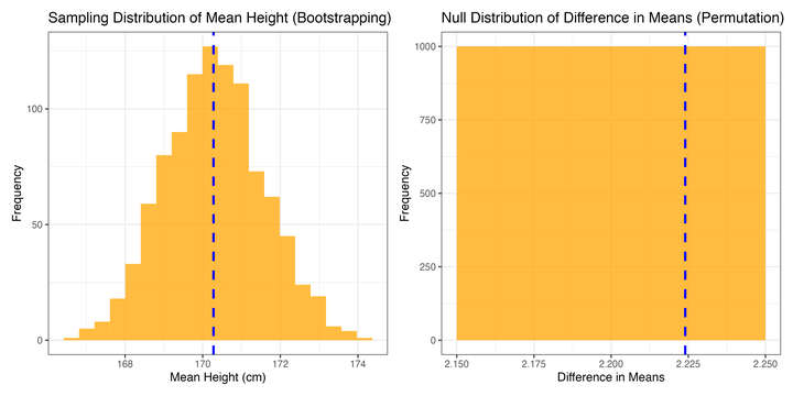
labs(title = "Sampling Distribution of Mean Height (Bootstrapping)",
x = "Mean Height (cm)", y = "Frequency") +
theme_bw()
p1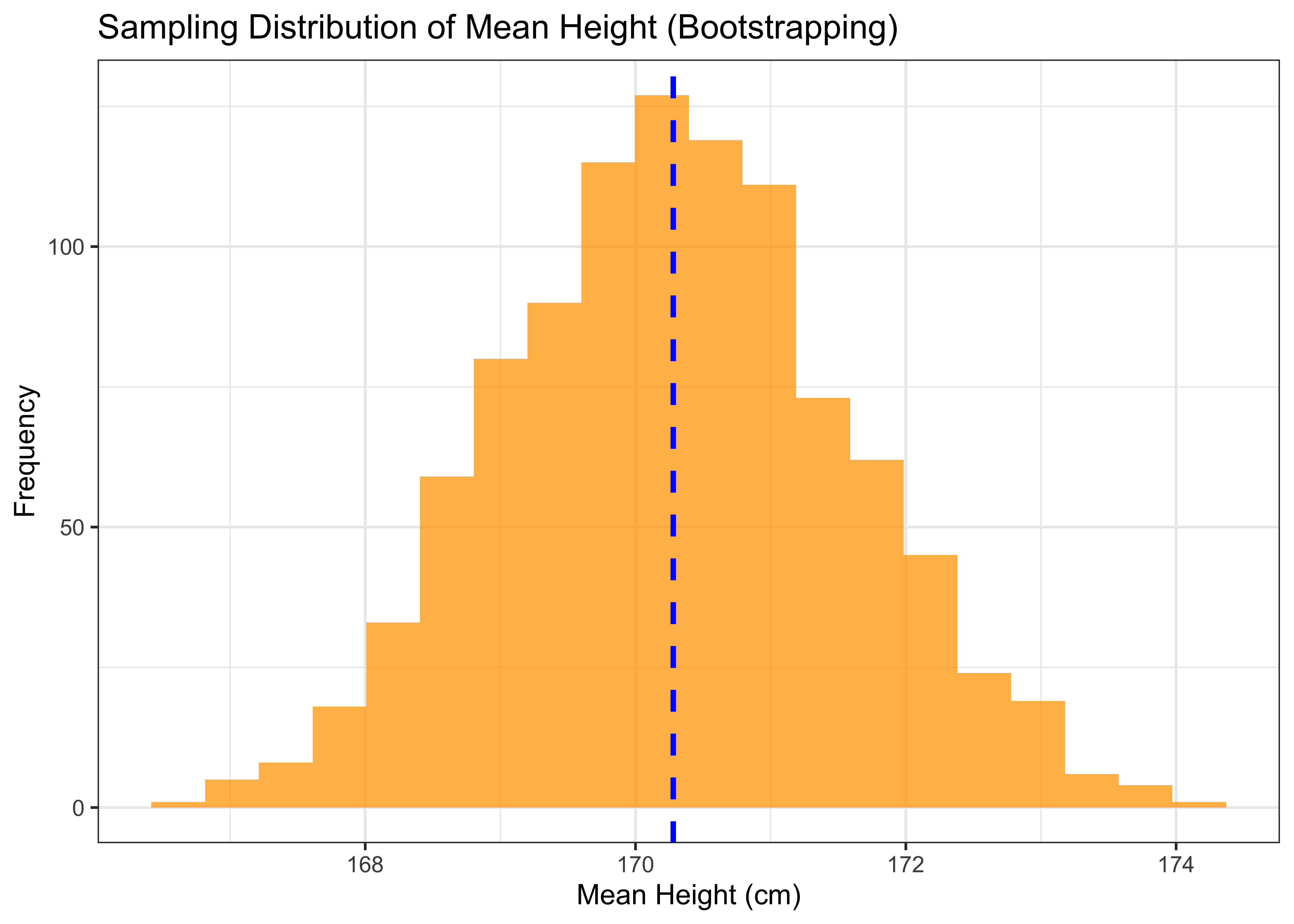
The output shows a bell-shaped curve that is centered around the estimated mean height of 170.3.
Permutation
Permutation, also known as randomization tests or exact tests, involves randomly shuffling the values of one or more variables and recalculating a statistic of interest. This is done repeatedly to create a null distribution of the statistic under the assumption of no association between the variables.
Permutation is often used when testing hypotheses about the relationship between variables or when comparing two groups. For example, suppose we are interested in whether there is a significant difference in the mean height between males and females. We can use permutation to test this hypothesis.
Let’s generate two samples of heights, one for males and one for females. We can visualize the null distribution of the F statistic using a density plot.
In this example, we first generate two random groups of data (group1 and group2) with means of 10 and 12, respectively. We then calculate the observed difference in means between the two groups.
We define a function diff_means that takes a list of two vectors and returns the difference in means between the two vectors. We then use this function with the replicate function to perform a permutation test and generate a null distribution of the difference in means between the two groups.
Finally, we create a histogram of the null distribution using ggplot, and we add a vertical line at the observed difference in means. This allows us to visually compare the observed difference in means to the null distribution of differences in means generated by the permutation test.
# Generate some random data for two groups
set.seed(123)
group1 <- rnorm(50, mean = 10, sd = 2)
group2 <- rnorm(50, mean = 12, sd = 2)

# Calculate observed difference in means
obs_diff <- mean(group2) - mean(group1)

# Define function to calculate difference in means between two groups
diff_means <- function(x) {
  return(mean(x[[2]]) - mean(x[[1]]))
}

# Use permutation to estimate null distribution of difference in means
perm_diff <-
  replicate(1000, diff_means(list(
    group1 = sample(group1), group2 = sample(group2)
  )))

# making dataframe
perm_diff <- data.frame(perm_diff)

# Create histogram of null distribution
p2 <- perm_diff |>
  ggplot(aes(x = perm_diff)) +
  geom_histogram(fill = "orange", alpha = 0.75, bins = 30) +
  geom_vline(xintercept = obs_diff, lty = 2, size = 1, color = "blue") +
  labs(title = "Null Distribution of Difference in Means (Permutation)",
       x = "Difference in Means", y = "Frequency") +
  theme_bw()

p2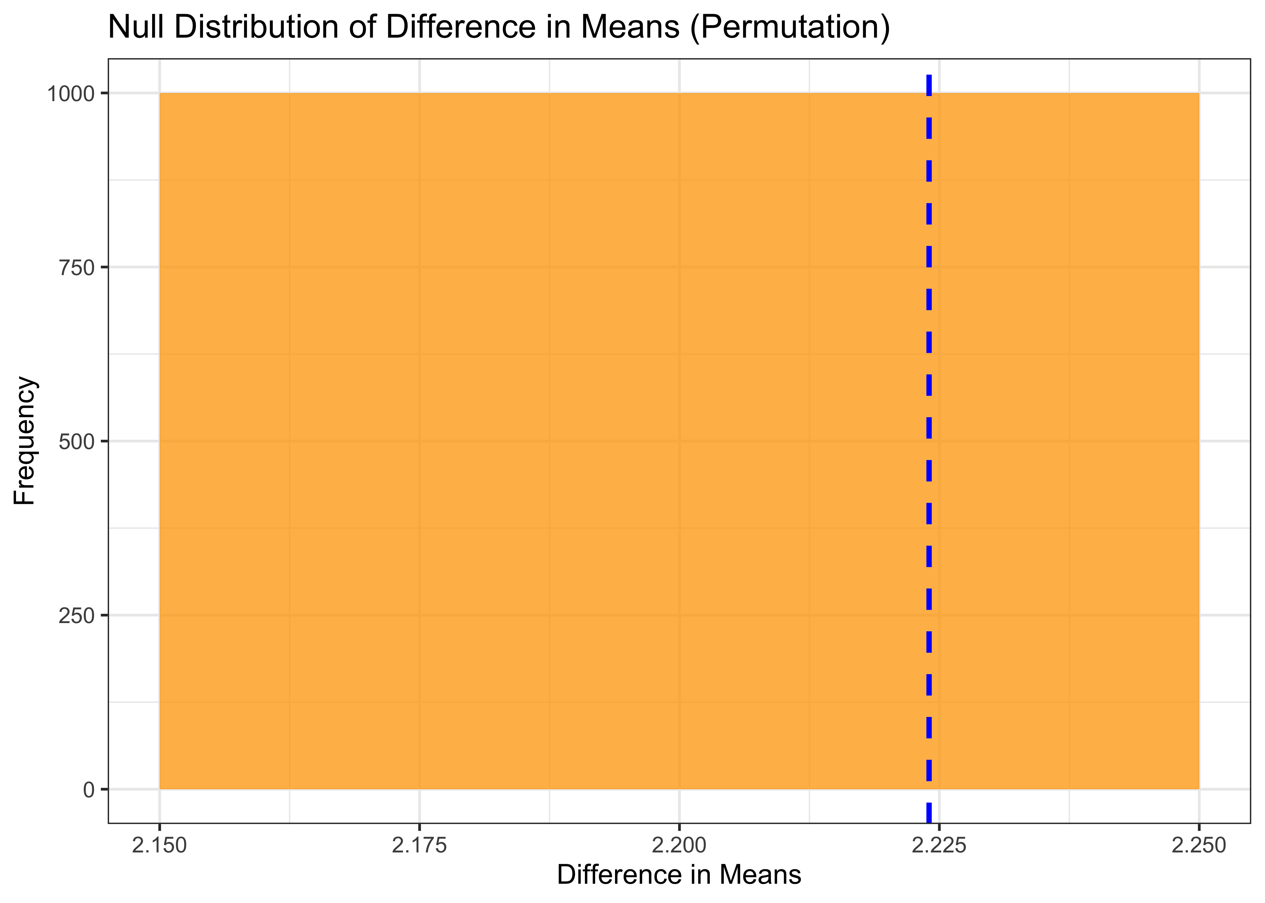
That’s it!
Feel free to reach me out if you got any questions.
Muhammad Mohsin Raza
Data Science Fellow
My research interests include disease modeling in space and time, climate change, GIS and Remote Sensing and Data Science in Agriculture.