Block Bootstrapping in R using Tidymodels

Last updated on Aug 24, 2022 10 min read Data Science

Often, we have situations where we want to bootstrap our analyses but in a way that all of the observations from a particular group (block) are randomly sampled than a mixture of observations from all groups. This can be achieved using block bootstrapping. Unfortunately, there is no easy or ready-made function available that can conduct block bootstrapping. However, we can use certain functions in base R and tidyverse packages to do this. In this blog post, I’ll show how we can perform block bootstrapping in R using tidyverse and tidymodels packages.

Load libraries

library(tidyverse)
library(tidymodels)
library(viridis)

Load data

For this blog post, I’ll use crop yield data from the UK from different study sites (locations) and years from 2002 - 2019. This data also contains monthly (Jan - Dec) weather data obtained from 2002 to 2019. So, let’s suppose we want to get the bootstrapped regression coefficient of the effect of temperature on the yield gap each month. And for this purpose, when bootstrapping data, we want to block the year information in a way that the data from one year is randomly sampled in each bootstrap rather than random rows from mixed years.

data <- read_csv("https://raw.githubusercontent.com/MohsinRamay/yieldgap/main/ww_wt.csv")
glimpse(data)

## Rows: 1,924
## Columns: 20
## $ ...1       <dbl> 1, 2, 3, 4, 5, 6, 7, 8, 9, 10, 11, 12, 13, 14, 15, 16, 17, …
## $ ID         <chr> "2002_Cirencester", "2002_Cirencester", "2002_Cirencester",…
## $ Year       <dbl> 2002, 2002, 2002, 2002, 2002, 2002, 2002, 2002, 2002, 2002,…
## $ Location   <chr> "Cirencester", "Cirencester", "Cirencester", "Cirencester",…
## $ Latitude   <dbl> 51.68076, 51.68076, 51.68076, 51.68076, 51.68076, 51.68076,…
## $ Longitude  <dbl> -1.9580083, -1.9580083, -1.9580083, -1.9580083, -1.9580083,…
## $ YieldTrt   <dbl> 9.642286, 9.642286, 9.642286, 9.642286, 9.642286, 9.642286,…
## $ YieldUntrt <dbl> 6.916857, 6.916857, 6.916857, 6.916857, 6.916857, 6.916857,…
## $ Mildew     <dbl> NA, NA, NA, NA, NA, NA, NA, NA, NA, NA, NA, NA, NA, NA, NA,…
## $ YellowRust <dbl> NA, NA, NA, NA, NA, NA, NA, NA, NA, NA, NA, NA, NA, NA, NA,…
## $ BrownRust  <dbl> 1.028571, 1.028571, 1.028571, 1.028571, 1.028571, 1.028571,…
## $ Septoria   <dbl> 21.151429, 21.151429, 21.151429, 21.151429, 21.151429, 21.1…
## $ gap        <dbl> 0.2822753, 0.2822753, 0.2822753, 0.2822753, 0.2822753, 0.28…
## $ Month      <chr> "September", "October", "November", "December", "January", …
## $ temp       <dbl> 13.646974, 13.336226, 7.065802, 3.442173, 5.610458, 6.92963…
## $ Date       <date> 2001-09-16, 2001-10-16, 2001-11-16, 2001-12-16, 2002-01-16…
## $ rh         <dbl> 81.12983, 87.08586, 86.82285, 85.21759, 89.50930, 82.90430,…
## $ sun        <dbl> 117.05141, 87.53126, 76.80444, 87.87857, 27.68811, 75.24004…
## $ rnf        <dbl> 39.70032, 95.11663, 40.74033, 21.97640, 78.55315, 102.96212…
## $ Season     <dbl> 2002, 2002, 2002, 2002, 2002, 2002, 2002, 2002, 2002, 2002,…

Study sites

Let’s plot the data on Map first to see the spatial distribution of study sites.

library(maps)
UK <- map_data("world") %>% 
  filter(region=="UK")

data %>% 
  distinct(Location, Longitude, Latitude) %>% 
  ggplot() +
  geom_polygon(data = UK, aes(x=long, y = lat, group = group), fill="grey", alpha=0.3, colour = "black") +
  geom_point(aes(x = Longitude, y = Latitude), colour = "steelblue") +
  coord_map() +
  labs(x = NULL, y = NULL, size = NULL, title = "Study sites", subtitle = "(2002 - 2020)") +
  theme_minimal() + 
  theme(plot.title = element_text(hjust = 0.5),
        plot.subtitle = element_text(hjust = 0.5))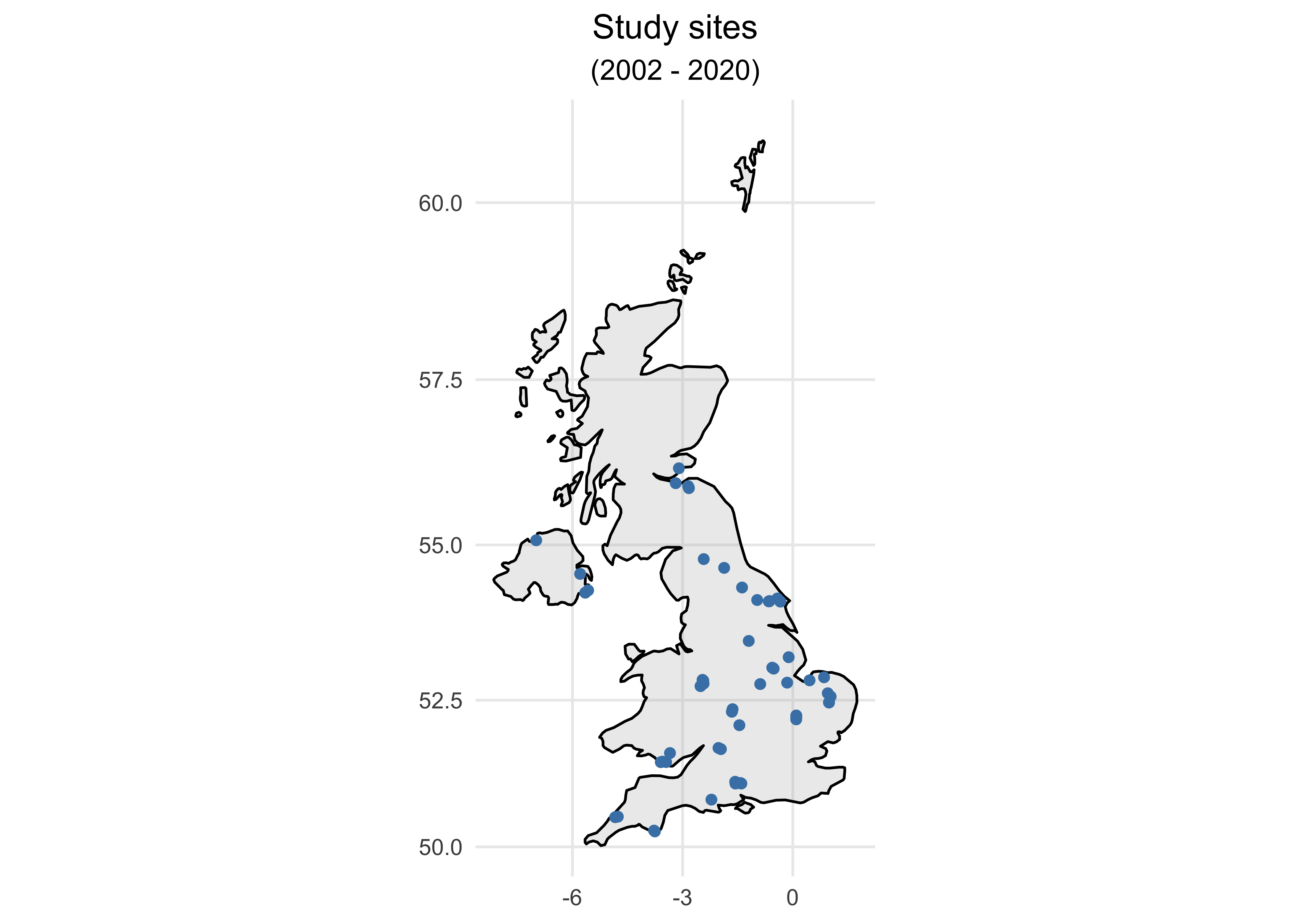

Block bootstrapping

First, I’ll select only those variables needed for final analysis, i.e., Year, Month, gap and temp.
- gap is the Yield gap, a variable of interest.

data %>% 
  ungroup() %>% 
  select(Year, Month, gap, temp)

## # A tibble: 1,924 × 4
##     Year Month       gap  temp
##    <dbl> <chr>     <dbl> <dbl>
##  1  2002 September 0.282 13.6 
##  2  2002 October   0.282 13.3 
##  3  2002 November  0.282  7.07
##  4  2002 December  0.282  3.44
##  5  2002 January   0.282  5.61
##  6  2002 February  0.282  6.93
##  7  2002 March     0.282  7.67
##  8  2002 April     0.282  9.42
##  9  2002 May       0.282 11.8 
## 10  2002 June      0.282 14.1 
## # … with 1,914 more rows
## # ℹ Use `print(n = ...)` to see more rows

Second, I’ll widen the temperature data by Months, so we have all data for a year at a specific study site in the same row.

data %>% 
  ungroup() %>% 
  select(Year, Month, gap, temp) %>%
  pivot_wider(names_from = Month, values_from = temp, values_fn = mean)

## # A tibble: 159 × 14
##     Year   gap Septe…¹ October Novem…² Decem…³ January Febru…⁴ March April   May
##    <dbl> <dbl>   <dbl>   <dbl>   <dbl>   <dbl>   <dbl>   <dbl> <dbl> <dbl> <dbl>
##  1  2002 0.282    13.6    13.3    7.07    3.44    5.61    6.93  7.67  9.42  11.8
##  2  2002 0.164    12.7    12.6    7.61    3.47    5.38    5.74  6.78  8.65  11.3
##  3  2002 0.226    13.3    13.6    7.02    3.59    5.04    6.74  7.42  9.26  12.3
##  4  2002 0.108    13.1    13.3    6.71    3.31    4.74    6.61  7.16  9.14  12.0
##  5  2002 0.311    12.9    12.9    6.69    3.01    4.83    6.51  7.17  8.98  11.6
##  6  2002 0.353    13.4    13.6    7.02    3.57    5.24    7.03  7.55  9.57  12.3
##  7  2002 0.268    13.2    13.0    7.36    3.14    5.03    6.82  7.40  9.00  11.8
##  8  2002 0.341    14.0    13.8    7.32    3.74    6.00    7.38  7.92  9.85  12.2
##  9  2002 0.309    13.4    13.9    7.05    3.40    5.11    6.91  7.46  9.35  12.2
## 10  2003 0.139    14.8    10.4    8.55    6.04    4.44    4.32  7.77  9.97  12.7
## # … with 149 more rows, 3 more variables: June <dbl>, July <dbl>, August <dbl>,
## #   and abbreviated variable names ¹September, ²November, ³December, ⁴February
## # ℹ Use `print(n = ...)` to see more rows, and `colnames()` to see all variable names

Third, I’ll use the bootstraps function from the rsample package to replicate data. The output will consist of a list of tibbles with bootstraps classes as id and a column for the data split objects.

data %>% 
  ungroup() %>% 
  select(Year, Month, gap, temp) %>%
  pivot_wider(names_from = Month, values_from = temp, values_fn = mean) %>% 
  bootstraps(times = 10, apparent = FALSE)

## # Bootstrap sampling 
## # A tibble: 10 × 2
##    splits           id         
##    <list>           <chr>      
##  1 <split [159/59]> Bootstrap01
##  2 <split [159/54]> Bootstrap02
##  3 <split [159/60]> Bootstrap03
##  4 <split [159/56]> Bootstrap04
##  5 <split [159/52]> Bootstrap05
##  6 <split [159/62]> Bootstrap06
##  7 <split [159/59]> Bootstrap07
##  8 <split [159/64]> Bootstrap08
##  9 <split [159/61]> Bootstrap09
## 10 <split [159/54]> Bootstrap10

Note: Here, I have used only 10 bootstrap replications. However, this number can be increased as per choice.

After that, I’ll use the map function to extract the data from each bootstrap split. It will return a list of tibbles where each tibble is a bootstrap sample.
I’ll then use the unnest function from the tidyr package to unnest tibbles to data frame.

data %>% 
  ungroup() %>% 
  select(Year, Month, gap, temp) %>%
  pivot_wider(names_from = Month, values_from = temp, values_fn = mean) %>% 
  bootstraps(times = 10, apparent = FALSE) %>% 
  mutate(splits = purrr::map(splits, analysis)) %>%
  unnest(splits)

## # A tibble: 1,590 × 15
##     Year     gap September October November December January Febru…¹ March April
##    <dbl>   <dbl>     <dbl>   <dbl>    <dbl>    <dbl>   <dbl>   <dbl> <dbl> <dbl>
##  1  2008 NA           14.9   11.2      7.25     5.31    7.09    5.44  6.71  8.73
##  2  2006 NA           16.1   13.9      6.35     4.46    4.30    4.21  5.17  9.19
##  3  2004  0.169       12.8    7.87     7.19     4.02    4.02    4.00  5.44  8.24
##  4  2005  0.0770      14.6   10.3      7.40     5.37    6.01    4.26  7.27  8.76
##  5  2016  0.218       12.1   10.4      8.97     9.49    4.82    4.52  4.91  7.05
##  6  2017  0.325       16.9   11.3      6.00     5.71    3.33    6.36  8.94  9.10
##  7  2017  0.340       16.7   11.2      5.92     5.73    3.45    6.35  8.91  9.22
##  8  2003  0.134       14.6    9.98     8.16     5.49    4.18    3.87  7.08  9.47
##  9  2014  0.446       14.6   13.1      6.79     6.37    6.14    6.71  8.13 10.5 
## 10  2010  0.217       13.4   11.5      7.76     3.40    2.82    2.90  5.95  9.01
## # … with 1,580 more rows, 5 more variables: May <dbl>, June <dbl>, July <dbl>,
## #   August <dbl>, id <chr>, and abbreviated variable name ¹February
## # ℹ Use `print(n = ...)` to see more rows, and `colnames()` to see all variable names

At this point, block bootstrapping has been done. However, we need the data in a long format for further data analysis and visualizations.
Therefore, I’ll use pivot_longer function to transform this wide data into the long format.
To keep track of observations in each bootstrapped sample, I’ll create a row ID before transforming the data to the long format.

set.seed(123)

# Block bootstrapping
boots <- data %>% 
  ungroup() %>% 
  select(Year, Month, gap, temp) %>%
  pivot_wider(names_from = Month, values_from = temp, values_fn = mean) %>% 
  bootstraps(times = 10, apparent = FALSE) %>% 
  mutate(splits = purrr::map(splits, analysis)) %>%
  unnest(splits) %>% 
  group_by(id) %>% 
  mutate(row = row_number()) %>% 
  pivot_longer(names_to = "Month", values_to = "temp", cols = September:August)

boots

## # A tibble: 19,080 × 6
## # Groups:   id [10]
##     Year    gap id            row Month      temp
##    <dbl>  <dbl> <chr>       <int> <chr>     <dbl>
##  1  2020 0.0979 Bootstrap01     1 September 15.2 
##  2  2020 0.0979 Bootstrap01     1 October   11.8 
##  3  2020 0.0979 Bootstrap01     1 November   8.15
##  4  2020 0.0979 Bootstrap01     1 December   7.54
##  5  2020 0.0979 Bootstrap01     1 January    7.37
##  6  2020 0.0979 Bootstrap01     1 February   7.65
##  7  2020 0.0979 Bootstrap01     1 March      7.89
##  8  2020 0.0979 Bootstrap01     1 April     12.0 
##  9  2020 0.0979 Bootstrap01     1 May       13.3 
## 10  2020 0.0979 Bootstrap01     1 June      15.0 
## # … with 19,070 more rows
## # ℹ Use `print(n = ...)` to see more rows

Visualize Block Bootstrapped Data

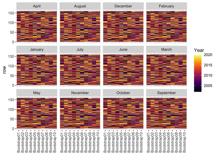
Now, we can visualize the bootstrapped data to check whether the data has been correctly bootstrapped, i.e., within each bootstrap, data from each Year is being randomly sampled with replacement.

# Bootstraps
boots %>%
  ggplot(aes(x = id, y = row, fill = Year)) +
  geom_tile() +
  scale_fill_viridis(option = "B", direction = 1) +
  labs(x = NULL) +
  facet_wrap(~Month) +
  theme(axis.text.x = element_text(angle = 90, hjust = 1, vjust = 0.4))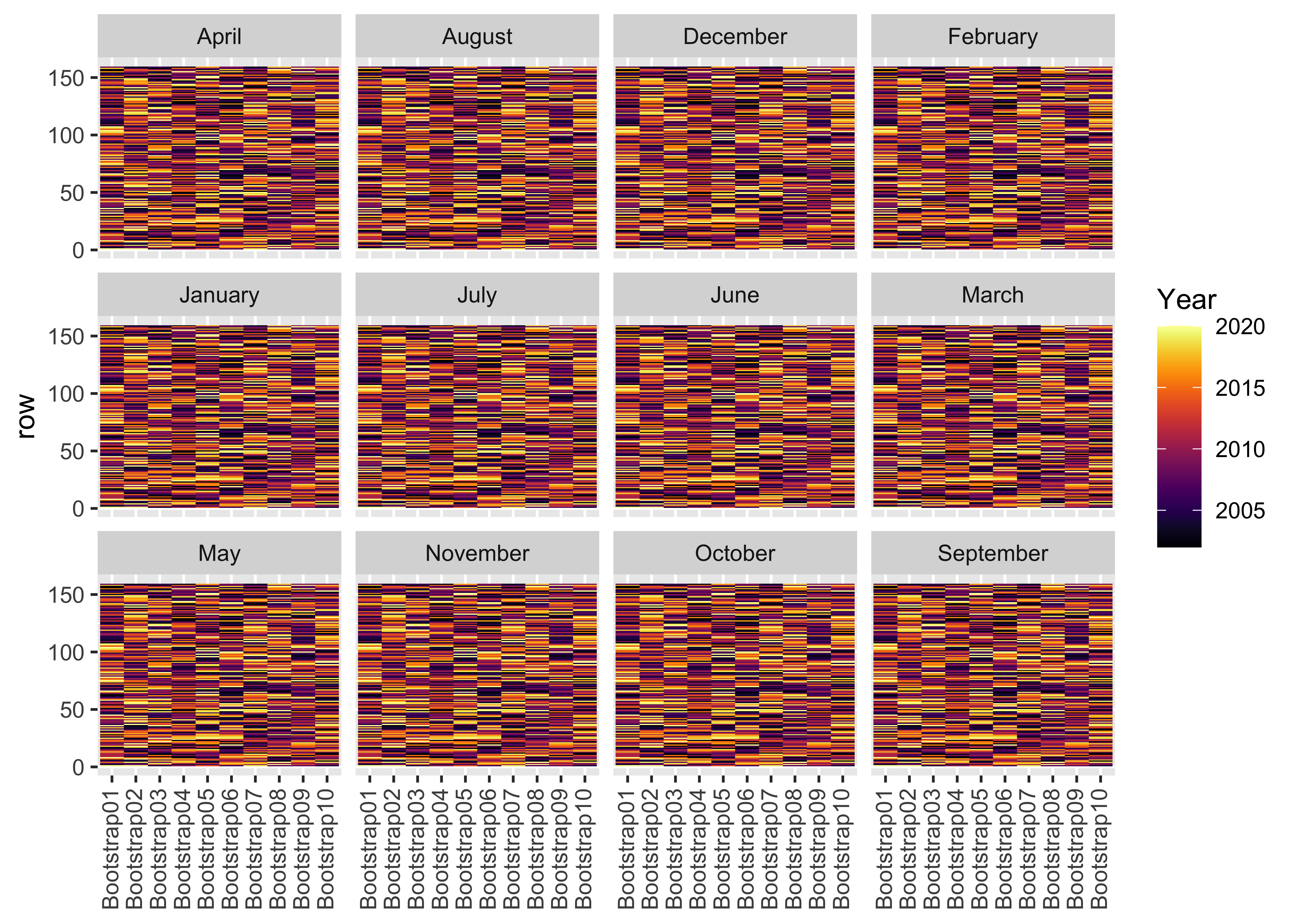

The above plots indicate that, within each bootstrap, data from each Year is being randomly sampled with replacement. Thus, we have bootstrapped data ready for subsequent analysis.

Regression Analysis

1000 bootstraps

I’ll rerun the block bootstrapping with 1000 replicates for regression analysis.

boots <- data %>% 
  ungroup() %>% 
  select(Year, Month, gap, temp) %>%
  pivot_wider(names_from = Month, values_from = temp, values_fn = mean) %>% 
  bootstraps(times = 1000, apparent = FALSE) %>% 
  mutate(splits = purrr::map(splits, analysis)) %>%
  unnest(splits) %>% 
  group_by(id) %>% 
  mutate(row = row_number()) %>% 
  pivot_longer(names_to = "Month", values_to = "temp", cols = September:August)

Model

I’ll use the tidymodels functionality to fit the regression model between yield gap and temperature.

boot_reg <- boots %>% 
  nest(data = -c(Month, id)) %>% # grouping the Month and Bootstrap samples
  mutate(model = purrr::map(data, ~lm(gap ~ temp, data = .x)), 
         coefs = purrr::map(model, tidy)) # performing regression
  
reg <- boot_reg %>% 
  unnest(coefs) %>% # unnesting tidied data frames
  select(-data, -id, -model)

reg

## # A tibble: 24,000 × 7
## # Groups:   id [1,000]
##    id            Month     term        estimate std.error statistic     p.value
##    <chr>         <chr>     <chr>          <dbl>     <dbl>     <dbl>       <dbl>
##  1 Bootstrap0001 September (Intercept)  0.261     0.104       2.50  0.0136     
##  2 Bootstrap0001 September temp        -0.00312   0.00750    -0.416 0.678      
##  3 Bootstrap0001 October   (Intercept)  0.0154    0.0572      0.269 0.789      
##  4 Bootstrap0001 October   temp         0.0186    0.00519     3.58  0.000466   
##  5 Bootstrap0001 November  (Intercept)  0.186     0.0417      4.46  0.0000164  
##  6 Bootstrap0001 November  temp         0.00446   0.00569     0.783 0.435      
##  7 Bootstrap0001 December  (Intercept)  0.108     0.0223      4.85  0.00000305 
##  8 Bootstrap0001 December  temp         0.0224    0.00422     5.30  0.000000421
##  9 Bootstrap0001 January   (Intercept)  0.105     0.0284      3.69  0.000313   
## 10 Bootstrap0001 January   temp         0.0249    0.00598     4.17  0.0000524  
## # … with 23,990 more rows
## # ℹ Use `print(n = ...)` to see more rows

Violin charts

I’ll use violin charts to plot the distribution of bootstrapped regression coefficients.

reg %>%
  filter(term == "temp") %>% 
  group_by(Month) %>%
  mutate(ci.95 = ifelse(estimate > quantile(estimate, 0.025) &  estimate < quantile(estimate, 0.975), "yes", "No")) %>% 
  mutate(Month = factor(Month, levels=c("September","October","November","December","January","February","March","April","May","June","July", "August"))) %>% 
  ggplot(aes(x = Month, y = estimate)) +
  geom_violin(draw_quantiles = c(.25, .50, .75), fill = "orange", alpha = 0.5) +
  geom_hline(yintercept = 0, lty = 2, colour = "red") +
  labs(x = NULL, y = "Bootstrapped estimates") +
  theme_test() +
  theme(axis.text.x = element_text(angle = 90, hjust = 1, vjust = 0.4))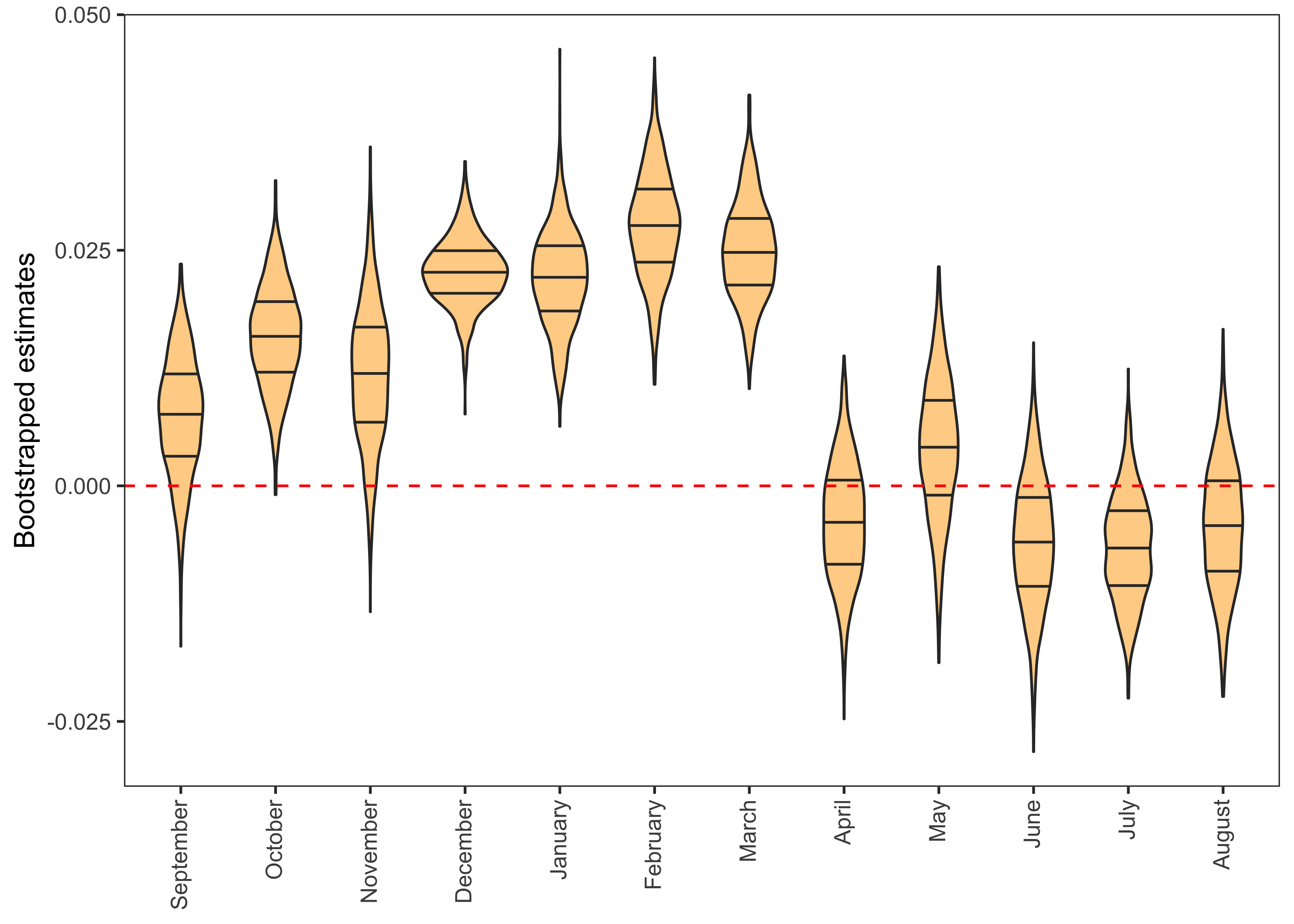

In this graph, Violin charts above the dashed red line indicate that temperature in the month of December, January, February and March has a significant positive relationship with the yield gap. This means that with rising winter temperature, the yield gap is also increasing, which is bad for food security. In other months, the distribution of bootstrapped estimates intersects the 0 line, thus indicating no statistically significant association.

That’s it!

Feel free to reach me out if you got any questions.

R bootstrapping block bootstrapping ggplot2 Data visualization